tutorial-01 - Flexible-fitting of an AlphaFold2 model into EMDB:23061
Hello, and thanks for your interest in TEMPy-ReFF! The purpose of this tutorial is to familiarise you with the basic aspects of running TEMPy-ReFF from the command line. We’ll focus on an “easy” refinement case, using an accurate AlphaFold model of the Ephydatia fluviatilis PiwiA-piRNA complex 1. We chose this example because the corresponding cryo-EM map (EMD-23061) is relatively small (90x90x90 voxels) and the AlphaFold model is reasonably accurate, so the TEMPy-ReFF refinements should run quite quickly.
The original model downloaded from the EBI AlphaFold2 database
(https://alphafold.ebi.ac.uk/entry/D5MRY8) is in
data/tutorial-01/original.pdb. A model which has had
terminal low-confidence regions trimmed and has been docked using
ChimeraX is in data/tutorial-01/docked.pdb, we’ll use this
as an input for refinement. The map from the EMDB
(https://www.ebi.ac.uk/emdb/EMD-23061) is in
data/tutorial-01/map.mrc.gz.
To simplify using RIBFIND2, we have precalculated secondary structure
prediction using DSSP. The output is in
data/tutorial-01/docked.dssp.
Step 0 - Get tutorial data and setup Conda environment
To download the tutorial data run the following command in the terminal:
git clone https://gitlab.com/topf-lab/tempy-reff-tutorials.git
cd tempy-reff-tutorials
Now, see if you have a conda environment set up already by running:
conda activate tempy_reff_envIf this fails, first create the environment:
conda env create -f tempy_reff_env.yml -n tempy_reff_envthen activate the environment, as shown above.
Step 1 - Visualising the starting model
Let’s take a look at the starting model, to get an idea of the kind of rearrangements required for successful refinement. We can open the model and cryo-EM map in ChimeraX with:
chimerax \
 data/tutorial-01/docked.pdb \
 data/tutorial-01/map.mrc \
You should see something like the image below (with some differences depending on your ChimeraX default parameters):
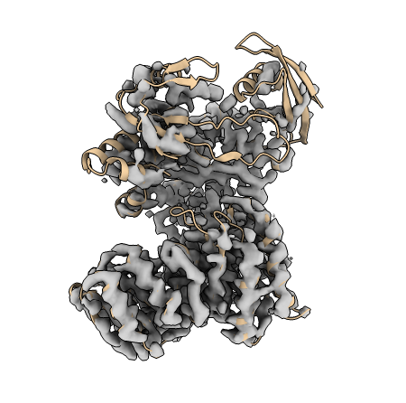
We can see that the AlphaFold model is a good fit within the bottom, higher resolution, portion of the map. However, towards the top of the map, the model is not such a good fit to the density. It looks like some clusters of alpha-helices and beta-sheets need to be rotated and rearranged to fit into the map. We can achieve this in TEMPy-ReFF with the help of RIBFIND restraints.
Step 2 - Run RibFind2
RIBFIND2 2 is a program for hierarchically clustering RNA and protein secondary structure elements together into “rigid-bodies”. For TEMPy-ReFF refinements, these rigid bodies are refined as single rigid units, rather than a collection of individual, flexible atoms. This can be very helpful in avoiding local minima during refinement, particularly when large rearrangements are required.
RIBFIND2 requires the model, and secondary structure annotations from DSSP (for proteins) or RNAview (for RNA). To simplify this tutorial, we will use pre-computed DSSP output. We can compute rigid bodies for the docked AlphaFold model with:
ribfind \
 --model data/tutorial-01/docked.pdb \
 --dssp data/tutorial-01/docked.dssp \
 --output-dir out/ribfind/tutorial-01
RIBFIND2 will output a series of “rigid body files” (text files defining the contents of each rigid body).
You run RIBFIND2 on your own complexes using the webserver here: https://ribfind.topf-group.com, and find instructions for installing RIBFIND locally here: https://ribfind.topf-group.com/download.
Step 3 - Run flexible fitting
With our RIBIND2 generated rigid bodies in hand, we can now run hierarchical flexible fitting with TEMPy-ReFF. When supplied with a directory containing multiple RIBFIND2 rigid bodies, TEMPy-ReFF will iteratively load the up the RIBFIND2 files, restrain atoms into rigid bodies, and run a round of refinement. This will start with the file containing the largest clusters, and sequentially reduce the cluster size.
We can start this process with the command below. This will result in
a directory out/flex-fit/tutorial-01 containing the output
of flexible fitting. The intermediate models are all stored, but the
final result will be called final.pdb.
tempy-reff \
 --model data/tutorial-01/docked.pdb \
 --map data/tutorial-01/map.mrc \
 --resolution 3.8 \
 --restrain-ribfind \
 --restrain-ribfind-dir out/ribfind/tutorial-01/protein \
 --fitting-density \
 --fitting-density-k 100 \
 --output-dir out/flex-fit/tutorial-01 \
 --platform-cuda
Whilst we wait for the run to complete we can explore some of these command line options in more detail:
Command line options
The first set of options (--pbd and --map)
simply control which files we use as input. We specify the cryo-EM map
resolution with the --resolution flag, which is 3.8 for
EMD-23061.
We trigger RIBFIND hierarchical refinement with the
--restrain-ribfind flag, and point TEMPy-ReFF to the
relevant RIBFIND files with the --restrain-ribfind-dir
flag. If we did not include the --restrain-ribfind flag,
TEMPy-ReFF would allow all atoms to move independently.
We can select which refinement force we use, using either the
--fitting-density or --fitting-gmm flags. The
fitting-force flag will instruct TEMPy-ReFF to use a
“density force” for refinement, where atoms will be pulled towards areas
with high cryo-EM density, similar to what is used in MDFF 3. The other option,
--fitting-gmm, uses the Gaussian-mixture model (GMM)
refinement approach that is described in the TEMPy-ReFF paper 4. Generally speaking, using the GMM
mode will produce better results but refinement will be significantly
slower than using the density force. Therefore, our general
recommendation is to run an initial round of flexible fitting with
RIBFIND2 restraints and the density force, to quickly fix larger errors,
and then correct any residual errors with a round of refinement using
the GMM, which is exactly what we’re doing here!
We can also tune the “strength” of our fitting force with the
--fitting-density-k parameter. In refinements using the
fitting density, the force applied to atoms is proportional the local
gradients in the cryo EM map, moving them to areas with high density
values. These gradients are typically small, meaning the forces applied
to atoms can be small, resulting in small, or even nonexistent, updates
to their position at each step. We can speed up refinements by
multiplying these gradients by a constant (i.e. the same for all atoms)
factor, which we control with the --fitting-density-k flag.
This parameter can require a bit of optimisation, but we generally found
100 to be a good starting point. If the refined model looks
quite deformed (i.e. high clashscore and many Ramachandran outliers),
try reducing this value. On the other hand, if refinement is taking ages
or the model doesn’t seem to be moving into obvious areas of density,
try increasing this value.
Finally, we can specify where the output files are stored with the
--output-dir flag, and where MD calculations are done with
either the --platform-cuda (for running the MD simulation
on a CUDA capable GPU) or --platform-cpu to do the
calculations on the CPU. If no platform is specified TEMPy-ReFF will try
and choose the best available platform.
Visualising the refined model.
When the refinement is finished we can visually assess how our model has improved with ChimeraX:
chimerax \
  data/tutorial-01/map.mrc \
  data/tutorial-01/docked.pdb \
  out/flex-fit/tutorial-01/final.pdb
Which, after setting the cryo-EM map threshold to 0.08, should look something like:
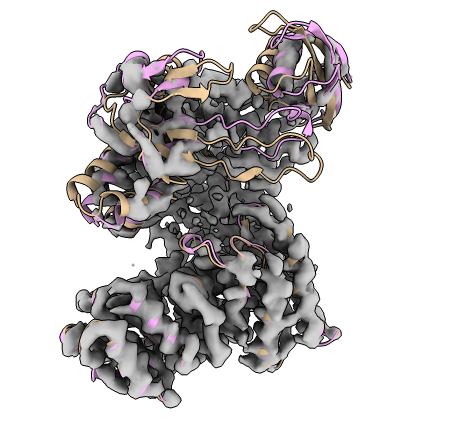
With our starting model in tan colouring, and our flexibly fit model shown in pink.
Quantifying the improvement in fit with SMOC
We can quantify these improvements using the SMOC score from TEMPy. The SMOC score evaluates the fit of each residue (or base for D/RNA) in our model, with a score between -1 and 1, with a higher score meaning a better fit. We installed TEMPy when we set up the conda environment, and we can calculate and plot the SMOC score with:
TEMPy.smoc \
  --models data/tutorial-01/docked.pdb out/flex-fit/tutorial-01/final.pdb \
  --map data/tutorial-01/map.mrc \
  -r 3.8 \
  --output-format png \
  --plot-type residue \
  --model-names "Starting Model" "Flexible Fitting Model" \
  --output-prefix out/flex-fit/tutorial-01/smoc
This will output a plot as a png image, in the same
out/flex-fit/tutorial-01/ directory where we stored our
flexibly fit models. If you locate this file
(out/flex-fit/tutorial-01/smoc_chain-A.png) and open it, it
should look something like this:
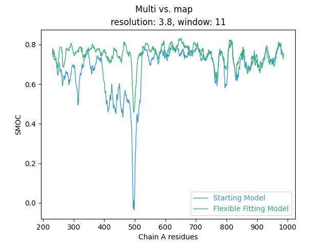
So we can see that our flexible fitting has lead to a significant improvement in model fit for residues 200 - 600. Let’s see if we can further improve the overall fit of the model using the more in depth GMM refinement.
Step 3 - GMM refinment
You may recall from earlier, that we can set up a GMM-based
refinement by passing the --fitting-gmm flag to TEMPy-ReFF.
We can set up a GMM-refinement using the output of flexible fitting
with:
tempy-reff \
 --model out/flex-fit/tutorial-01/final.pdb \
 --map data/tutorial-01/map.mrc \
 --resolution 3.8 \
 --fitting-gmm \
 --fitting-gmm-k 5e4 \
 --convergence-type patience \
 --convergence-timeout 100 \
 --output-dir out/refine/tutorial-01 \
 --platform-cuda
Again, whilst we wait for the refinement to finish, we can explore some the new command line arguments we just used to run our refinement.
GMM command line arguments
In addition to the --fitting-gmm flag we supplied to
trigger GMM based refinement, we also needed to include the
--fitting-gmm-k flag, which sets the strength of our
fitting force. This is an important parameter which essentially defines
how hard each atom is pulled in the direction the GMM believes it should
go. Occasionally, it is necessary to manually tune this fitting force,
as too low a force can result in too little bias being placed on the
cryo-EM data, and essentially an under-fit model, whereas, when the
fitting force is set too high the model can overfit and become
distorted, leading to increases in Ramachandran outliers and clashes.
Generally, we’ve found 5e4 to be a good starting value for
an initial refinement. If you feel that your model is not moving into
obvious cryo-EM density, try increasing the fitting force by, say, a
factor of 2. Conversely, if your model is starting to become distorted,
try reducing the fitting force.
Some extra new parameters are --convergence-type and
--convergence-timeout, which both control when and why
TEMPy-ReFF will stop refinements. TEMPy-ReFF has two methods for
determining when a refinement has completed, one which measures the
variance in a scoring function (normally the CCC between the model and
cryo-EM map) and another which monitors whether this scoring function is
improving or not. For the flexible-fitting refinement, we used the
variance measure, which can be manually set with
--convergence-type variance, although this is the default
option. However, for the GMM refinement it can be worth using the
--convergence-type patience option. The “patience”
approach, checks if the CCC between the map and model is improving, and
terminates the refinement if it does not improve for a set number of
steps (the number of steps is 5 by default, but can be manually set with
the --convergence-patience flag, i.e. to wait 10 steps
before stopping refinement use: --convergence-patience 10).
The patience method can be advantageous for the GMM refinement as
sometimes the model will only improve a little between steps, and the
variance between these values can fall below the threshold for stopping
the refinement even though the model is still improving. Finally, there
is the --convergence-timeout flag. This sets the maximum
number of steps to run before just stopping refinement. In our case we
stopped after 100 steps, even though the model was still improving. We
could probably squeeze out some further improvements with more steps,
but this is probably enough to illustrate what kind of improvements you
can expect with the GMM refinement.
Quantifying the improvement in fit with SMOC
We can again quantify our improvement in fit using the SMOC score. For reference, we will include both our starting AlphaFold model, and the output from flexible fitting, that we used as input for this refinement.
TEMPy.smoc \
  --models data/tutorial-01/docked.pdb \
           out/flex-fit/tutorial-01/final.pdb  \
           out/refine/tutorial-01/final.pdb  \
  --map data/tutorial-01/map.mrc   \
  --resolution 3.8  \
  --output-format png  \
  --plot-type residue  \
  --model-names "Starting Model" "Flexible Fitting Model" "GMM Refined Model" \
  --output-prefix out/refine/tutorial-01/smoc
Again, we output the plot as a png file into the directory with our
saved models (the file is named:
out/refine/tutorial-01/smoc_chain-A.png). If we view the
plot we can see that the GMM refinement has further improved the model
fit:
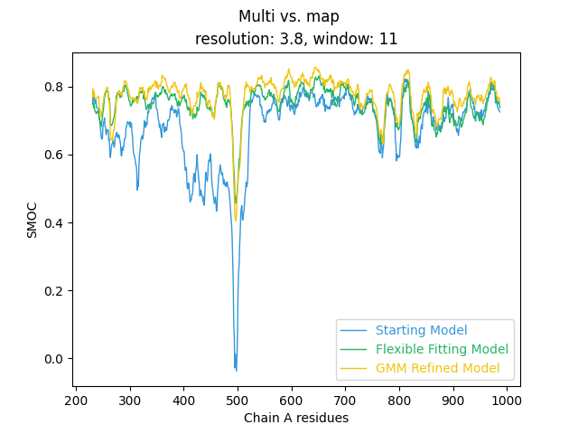
However, we don’t see another massive improvement in the SMOC score, similar to what we observed with flexible fitting. That’s primarily because our flexibly fit model was already a reasonable fit to the cryo-EM map, and the GMM refinement just needed to fix some remaining small errors.
Visualising the refined model.
We can visualise the changes to our model, using ChimeraX:
chimerax \
  data/tutorial-01/map.mrc \
  out/flex-fit/tutorial-01/final.pdb \
  out/refine/tutorial-01/final.pdb
This time, lets view all the atoms (rather than just secondary
structure), using either the command show all or clicking
the Show Atoms button on the toolbar. TEMPy-ReFF models
contain hydrogen atoms, which are required for the openMM simulations.
These can make viewing the models a little messy, so we can hide them
using the hide H command. You should see something like
this:
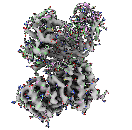
with the flexible fitting model in pink, and the GMM refined model in green. Similar to what we observed in the SMOC plot, we only see subtle changes after refinement.
Summary
To summarise, we recommend the following workflow for most model fitting problems, particularly those starting from AlphaFold predictions:
- Run a round of flexible fitting with RIBFIND2 restraints.
- Refine this flexibly fit model using a GMM refinement.
Furthermore, we strongly recommend using --platform-cuda
for refinements (i.e. using the GPU for calculations), where possible.
This is much, much faster than using the CPU. If no platform argument is
specified, TEMPy-ReFF will try and use the best available platform.
Flexible fitting recommendations:
For flexible fitting refinements (i.e. those using RIBFIND restraints), we recommend starting with:
--convergence-type varianceas the large rearrangements in flexible fitting will often result in large CCC improvements.--fitting-densityas the density fitting force is much faster than the GMM, which updates the models in much smaller steps- Starting with a
--fitting-density-kvalue of100.0, and decreasing this if the output model is badly deformed (high clashscore, many Ramachandran outliers)
GMM Refinement recommendations:
For GMM refinements we recommend starting with:
--convergence-type patienceas the small adjustments done by the GMM refiner between steps can result in a very low variance in CCC between steps, leading to refinements stopping too early.- Starting with a
--fitting-density-gmmvalue of5e4, and, as above, decreasing this if the output model is badly deformed (high clashscore, many Ramachandran outliers)
References
Anzelon, T.A., Chowdhury, S., Hughes, S.M. et al. Structural basis for piRNA targeting. Nature 597, 285–289 (2021). https://doi.org/10.1038/s41586-021-03856-x↩︎
Malhotra, S., Mulvaney, T., Cragnolini, T. et al. RIBFIND2: Identifying rigid bodies in protein and nucleic acid structures, Nucleic Acids Research, Volume 51, Issue 18, 13 October 2023, Pages 9567–9575, https://doi.org/10.1093/nar/gkad721↩︎
Trabuco LG, Villa E, et al. Flexible fitting of atomic structures into electron microscopy maps using molecular dynamics. Structure. 2008 May;16(5):673-83. doi: 10.1016/j.str.2008.03.005. PMID: 18462672; PMCID: PMC2430731.↩︎
Beton, J.G., Mulvaney, T., Cragnolini, T. et al. Cryo-EM structure and B-factor refinement with ensemble representation. Nat Commun 15, 444 (2024). https://doi.org/10.1038/s41467-023-44593-1↩︎